1. Introduction
The human will to register the relevant information that he has been building over centuries goes necessarily through the two-dimensional representation of the three-dimensional visual information he receives. Thus, to obtain a two-dimensional representation of the earth we must found a bijective correspondence between points on a plane and points on a sphere that preserve certain relationships.
These relationships are a crucial factor to decide which representation we want to follow. Regarding navigation angle-preserving maps projections are quite suitable and when artic regions are involved it would be also desirable to have the following additional properties: identification of meridians and parallels to rays and circles, respectively. As we shall see the stereographic projection is a projection with these properties. In fact, it is the only projection map that identifies small circles in the sphere with planar circles.
Our aim is the creation of a flexible GeoGebra tool, the PRiemannz tool, which identifies the spherical point set in correspondence, via the stereographic projection, to a given particular set of planar points. This tool acts as an invaluable aid in the understanding of the fundamental stereographic projection properties, being also a privileged tool in revealing the amazing correspondence between Möbius transformations and motions of the sphere.
For this purpose we have organized the following sections of this paper as follows: section 2 is devoted to theoretic aspects of the Riemannian sphere and of the stereographic projection and its fundamental properties. One of it´s main properties will be described (straight lines and circles are projections of spherical circles); in section 3 we will describe the main functionalities of the PRiemannz tool and in section 4 we will present a preliminary application of PRiemannz tool in order to illustrate some of the properties of mobius transformations.
2. Stereographic Projection and the Riemannian Sphere
To define a stereographic projection of the unit sphere 


Let us begin by taking the equatorial plane as the projection plane, let N is the point of the ball is farthest from the projection plane. In this case, the stereographic projection 


Looking at the analytical expression of 


3. The PRiemannz tool  .
.
Let us now see how we may express, dynamically, the action of a stereographic projection map in GeoGebra.
In GeoGebra we may represent the Argand plane in a 2d window, using the tool point ( with the option complex number), or writing directly in the command bar a complex in the algebraic form. If we write, for instance, 2-3i we see the affix z1 in the 2d view and z1= 2-3i in the a algebraic window.
Several characteristic of the complex number z1, such as, its real part [real(z_1)], its imaginary part [imaginary(z_1)], its argument [arg(z_1)] and its module [abs(z_1)] can be easily obtained.
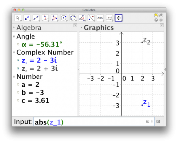
Figure 1 – View of GeoGebra application, Algebra and Graphic Windows. The Graphic Window corresponds to the Argand Plane.
Instead of working directly with the stereographic projection we have used its inverse map considering the Argand plane as the projection plane and (0,0,1) as the projection point to created the PRiemannz tool . How does it work?
Given a complex number z_1=1+i, the PRiemannz tool plots the spherical point RS(z1) whose image by the stereographic projection, in consideration, is exactly z_1. The point in the sphere is given, as expected, by Intersect[Segment[(0, 0, 1), z_1], Sphere[(0, 0, 1), 1], 2].
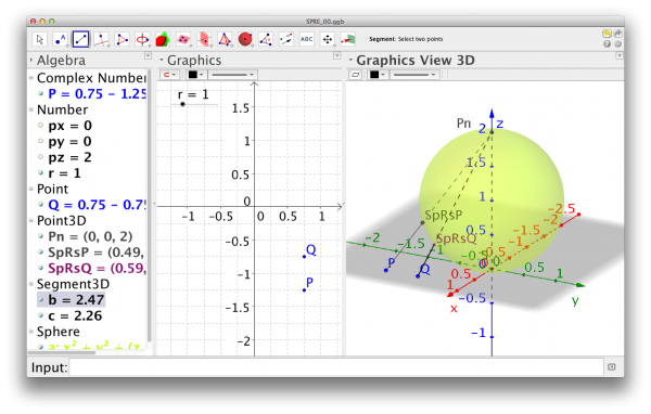
Figure 2 – View of GeoGebra application, point in Argand plane and its corresponding spherical point.
Looking at the identification, via the stereographic projection in consideration, we realize that: the unit circle 


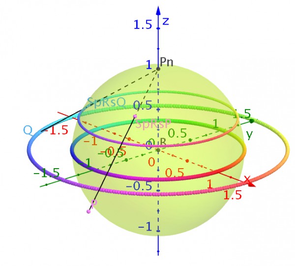
Figure 3 – Action of stereographic projection on the frontier, interior and exterior of the complex unit disc.
Let us make some explorations with the PRiemannz, tool about the action of 
To do this, in the case of concentric circles, we consider a region, in the Argand plane, given by a list, for example, CpA=Sequence[Circle[(0, 0), i], i, 1, n, 1] and observe what happens to the correspondent points in the Sphere, which are given by Sequence[PRiemann[Point[CpA, i]], i, 0, 1, 0.001] (fig.4). Soon, we realize that we are in presence of spherical circles that are spherical parallels, when the center of the circles corresponds to the complex 
These explorations lead us to the conjecture that concentric circles and straight lines passing through the origin correspond to stereographic projections of spherical circles being that the latter are projections of spherical circles passing through the North Pole.
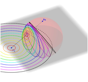
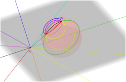
Figure 4 – Action of stereographic projection on concentric circles and straight lines passing through the origin.
In fact, the plane Π with equation Ax+By+Cz=D will intersect S2 in a circle if A2+B2+C2>D2. Now, the spherical point corresponding to z=x+iy is

which lies in the plane Π if and only if 2Ax+2By+C(x2+y2-1)=D(1+x2 +y2). That is, if and only if (C-D)(x2+y2)+2Ax+2By+(-C-D)=0 (*) which represents the equation of a circle in the complex plane if C≠D with center(A/(D-C), B/(D-C)) and radius 
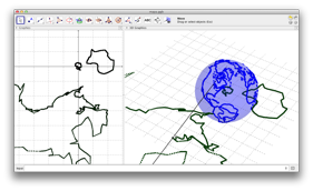
Figure 5 – Application of stereographic projection in cartography using GeoGebra.
Cartography is one example where the properties of the stereographic projection are applied. With the tool we have created, several types of planar maps may be obtained (see figure 5). This is one of the most popular applications of the stereographic projection. In the next section we will apply the stereographic projection of the Riemann sphere to study some of the properties of the Möbius Transformations.
4. The Möbius Transformations and some properties
A Möbius Transformation is a map of the extended complex plane 


 ,
, 
The Möbius Transformations under composition form a group generated by: translations,


In the complex plane, the equation 
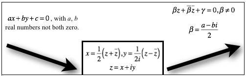
Figure 6
Moreover the equation 


4.1 Study the Möbius Transformation in GeoGebra, concentric circles and radial segments.
First we need to start with four parameters a, b, c and d such as ab≠cd. Let a=1, b=1, c=1 and d=-1 in the input bar. Considering the complex numbers z_1 and z_2 the Möbius Transformation gives:
MTz_1= (a z_1+b)/(c z_1+d) and MTz_2=(a z_2+b)/(c z_2+d).
For example if z_3=Midpoint[z_2, z_1] it is easy obtain the Möbius Transformation of the midpoint of a segment s, defined by z_1 and z_2, it is MTz_3=(a z_3+b)/(c z_3+d). Using locus of a point P in the segment s and view the trace of MTP we can observe that the Möbius transformation of s is an arc of circle, MTs (fig. 7).
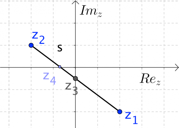
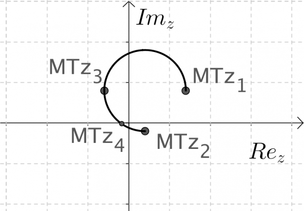
Figure 7 – Images of sets of complex numbers, at left, for MT(1,1,1,-1), at right.
This fact allows us to obtain, in general, the Möbius Transformation of the segment z_1 z_2 using the sequence of commands:
MTz_3=(a z_3+b)/(c z_3+d) ;
CircumcircularArc[(a z_1 + b) / (c z_1 + d), (a z_3 + b) / (c z_3 + d), (a z_2 + b) / (c z_2 + d)].
However, it is necessary to do it with caution and use an algebraic expression for MTz_3 in the command line. Now, we will see how to get the images of concentric circles and segments by the Möbius Transformation of parameters a,b, c and d .
In GeoGebra we can create the concentric circles and segments using the command list and type in the input bar something similar to:
CC=Sequence[Circle[(real(z_{CC}), imaginary(z_{CC})), k l / n], k, 1, n, 1] ;
RC=Sequence[Rotate[Segment[(real(z_{RC}), imaginary(z_{RC})),(real(z_{RC})+l, imaginary(z_{RC}))], j 2 π / n, (real(z_{RC}), imaginary(z_{RC}))], j, 0, n, 1] .
Using a free point in the list, z_P=Point[RC], the Möbius Transformation of this point is:
MTz_P = (az_P+b)/(cz_1+d),
and the locus leads to the image of the list of the Möbius Transformation. In fact circles are sent to other circles (fig. 8).
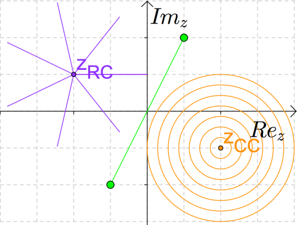
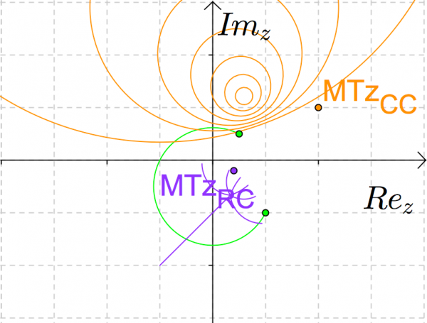
Figure 8 – Images of sets of complex numbers, at left, for MT(1,1,1,-1), at right.
Using the 3D capacities of GeoGebra we can vizualize the effects of Möbius transformations of the Riemann Sphere on these set of objets using the PRiemannz tool. The images below show the projection in the Riemann sphere of the sequences of concentric circles, rays, as well as, the effect in the Riemann sphere namely, translations, rotations (along the axis), and dilation via Möbius Transformation. In fact the mobius transformation preserves the Riemann sphere (fig. 9).
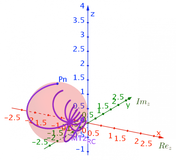

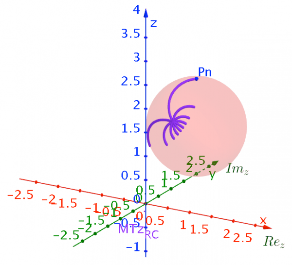
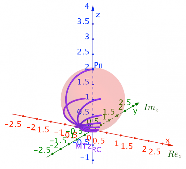
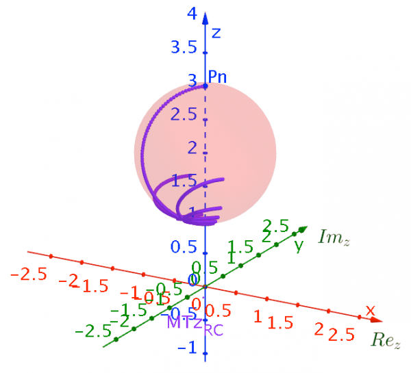
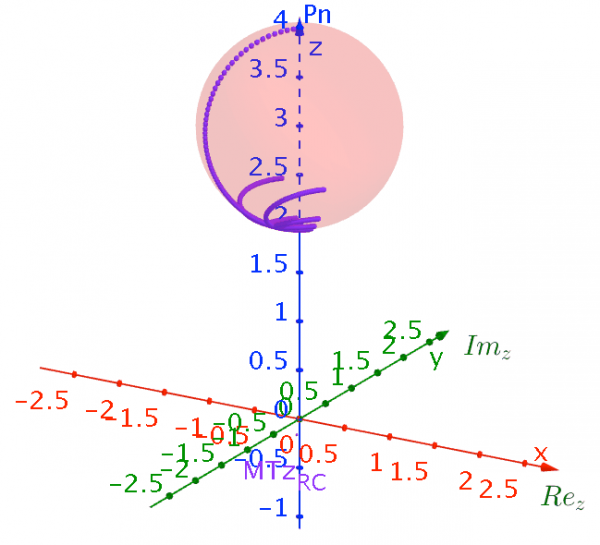
Figure 9– Effects of rotations, along imaginary axis, and translation, along z axis, of the Riemann sphere via Möbius Transformation.
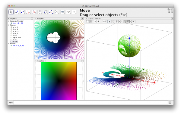
Using both the PRiemannz tool and the coloring domain technique (Breda, A. Santos, J. 2013) we may show the action of the Möbius transformations on the extended complex plane. In figure 10 some interesting features can be seen relating motions of the Riemann sphere and Möbius Transformations.
 |
 |
Figure 10 – Application of domain coloring using GeoGebra to visualize Riemann sphere and Möbius Transformations.
This is all we can do with the most recent version of GeoGebra 4.9 .The next step of our research is the identification of the improvements that should be performed in GeoGebra to visualize effectively the action of the Möbius Transformation in the Riemann sphere. Our future goals are the production of some images and videos regarding an improvement in the vizualitation of the motions of the Riemannian Sphere as it is done in the paper and in the video “Möbius transformations revealed”, brilliantly described by Douglas N. Arnold and Jonathan Rogness, published by Notices of the AMS. This improvement will mean that we could use GeoGebra to vizualize and study all kind of maps of the complex plane into the complex plane, looking at the graphs of these maps in the Riemann sphere.
Conclusions
In this paper we show how we can use the GeoGebra to study the stereographic projection, as well as, the application of this technique to the study of some properties of the Riemann Sphere and the Möbius Transformation. We have exposed how GeoGebra can be used in these topics of non-trivial mathematics issues and the benefits of the visualization for teaching in high school level.
Some improvements in the software must be done to produce better images and videos, in order to obtain a good visualization of the effects of geometric transformation in the Riemann Sphere. In future versions, it is necessary to collect the color information of the locus of points in 3D to save patterns in the sphere surface of a new object. We can also apply geometric transformations to explore mathematical relations.